本章學習目標
前面幾章我們常常處理平均值:血壓平均下降多少、LDL-C 平均差多少、住院天數平均是否改變。不過醫學研究裡有很多問題不是連續數值,而是「有或沒有」、「陽性或陰性」、「死亡或存活」、「接種或未接種」。
這些資料稱為類別資料 (categorical data)。如果類別只有兩種,例如是否再住院,就稱為二元資料 (binary data)。處理這類資料時,我們關心的通常是比例 (proportion)、風險 (risk)、勝算 (odds),以及不同組別之間是否有關聯。
讀完本章後,你應該能夠:
- 區分類別資料、二元資料與有序類別資料。
- 使用單一比例檢定 (one-sample proportion test) 與兩比例 z 檢定 (two-proportion z test)。
- 使用卡方獨立性檢定 (chi-square test of independence) 分析列聯表。
- 在小樣本或稀有事件時使用 Fisher exact test。
- 使用 McNemar test 分析配對二元資料。
- 對有序類別資料進行趨勢檢定 (trend test)。
- 報告類別資料分析時同時呈現效果大小與 p 值。
類別資料的基本語言
類別資料的第一個重點是計數。假設 420 位對照組病人中有 52 位發生不良事件,這不是平均值問題,而是「52/420」這個比例是否太高、是否和另一組不同。
常見的量包括:
- 風險 (risk):事件發生人數除以總人數。例如 52/420。
- 勝算 (odds):事件發生人數除以未發生人數。例如 52/368。
- 風險差 (risk difference):兩組風險相減。
- 相對風險 (relative risk):兩組風險相除。
- 勝算比 (odds ratio):兩組勝算相除。
風險比較直覺,勝算比在病例對照研究與 logistic regression 中很常見。剛開始學時,先不要把 odds ratio 自動解讀成 relative risk;事件常見時,兩者可以差很多。統計不怕你慢慢來,怕的是我們太快把它們當成同一個東西。
單一比例檢定
單一比例檢定用於檢查某個樣本比例是否與一個已知或假設比例不同。例如某醫院過去 30 天再住院率為 12%,新的照護計畫後觀察到 200 位出院病人中有 18 位再住院。研究者想問:新的再住院率是否低於 12%?
在 R 中,可使用 binom.test。它直接根據二項分布計算 p 值,對小樣本也很合適。
readmit_events <- 18
readmit_total <- 200
historical_rate <- 0.12

one_prop_result <- binom.test(readmit_events, readmit_total, p = historical_rate, alternative = "less")

one_prop_df <- data.frame(
  quantity = c("觀察再住院率", "歷史再住院率", "單尾 p 值"),
  value = c(readmit_events / readmit_total, historical_rate, one_prop_result$p.value),
  stringsAsFactors = FALSE
)
one_prop_df$value <- round(one_prop_df$value, 4)

one_prop_df
      quantity  value
1 觀察再住院率 0.0900
2 歷史再住院率 0.1200
3    單尾 p 值 0.1129
這裡的虛無假設是再住院率等於 12%,對立假設是再住院率低於 12%。如果研究者事前沒有方向性假設,應使用雙尾檢定。
兩比例 z 檢定
兩比例 z 檢定用於比較兩個獨立組別的比例。它依賴常態近似,因此各組事件與非事件數不宜太小。若格子數很小,後面會介紹 Fisher exact test。
範例 1:疫苗組不良事件比例是否較低?
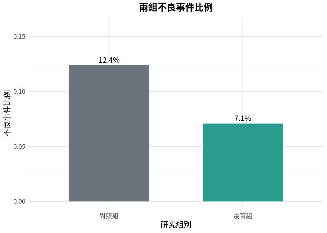
假設一項研究比較疫苗組與對照組的不良事件比例。對照組 420 人中有 52 人發生不良事件;疫苗組 438 人中有 31 人發生不良事件。
control_events <- 52
control_total <- 420
vaccine_events <- 31
vaccine_total <- 438

prop_df <- data.frame(
  group = c("對照組", "疫苗組"),
  events = c(control_events, vaccine_events),
  total = c(control_total, vaccine_total),
  stringsAsFactors = FALSE
)
prop_df$risk <- prop_df$events / prop_df$total
prop_df$group <- factor(prop_df$group, levels = c("對照組", "疫苗組"))

prop_df
   group events total       risk
1 對照組     52   420 0.12380952
2 疫苗組     31   438 0.07077626
p1 <- ggplot(prop_df, aes(x = group, y = risk, fill = group)) +
  geom_col(width = 0.6, show.legend = FALSE) +
  geom_text(aes(label = sprintf("%.1f%%", risk * 100)), vjust = -0.5, size = 4) +
  scale_fill_manual(values = c("對照組" = "#6c757d", "疫苗組" = "#2a9d8f")) +
  scale_y_continuous(limits = c(0, 0.16)) +
  labs(
    title = "兩組不良事件比例",
    x = "研究組別",
    y = "不良事件比例"
  )

p1
two_proportion_z_test <- function(success_a, total_a, success_b, total_b) {
  p_a <- success_a / total_a
  p_b <- success_b / total_b
  pooled <- (success_a + success_b) / (total_a + total_b)
  se <- sqrt(pooled * (1 - pooled) * (1 / total_a + 1 / total_b))
  z_stat <- (p_a - p_b) / se
  p_value <- 2 * (1 - pnorm(abs(z_stat)))
  return(list(z_stat = z_stat, p_value = p_value, risk_diff = p_a - p_b))
}

z_res <- two_proportion_z_test(vaccine_events, vaccine_total, control_events, control_total)

two_prop_test_df <- data.frame(
  quantity = c("疫苗組風險", "對照組風險", "風險差", "z 統計量", "雙尾 p 值"),
  value = c(vaccine_events / vaccine_total, control_events / control_total, z_res$risk_diff, z_res$z_stat, z_res$p_value),
  stringsAsFactors = FALSE
)
two_prop_test_df$value <- round(two_prop_test_df$value, 4)

two_prop_test_df
    quantity   value
1 疫苗組風險  0.0708
2 對照組風險  0.1238
3     風險差 -0.0530
4   z 統計量 -2.6270
5  雙尾 p 值  0.0086
p 值回答的是「若兩組真實比例相同,看到這麼極端或更極端資料的機率有多大」。但臨床判讀還需要看風險差。若風險差是 -5.3 個百分點,這比單看 p 值更接近病人與決策者真正關心的問題。
列聯表與卡方獨立性檢定
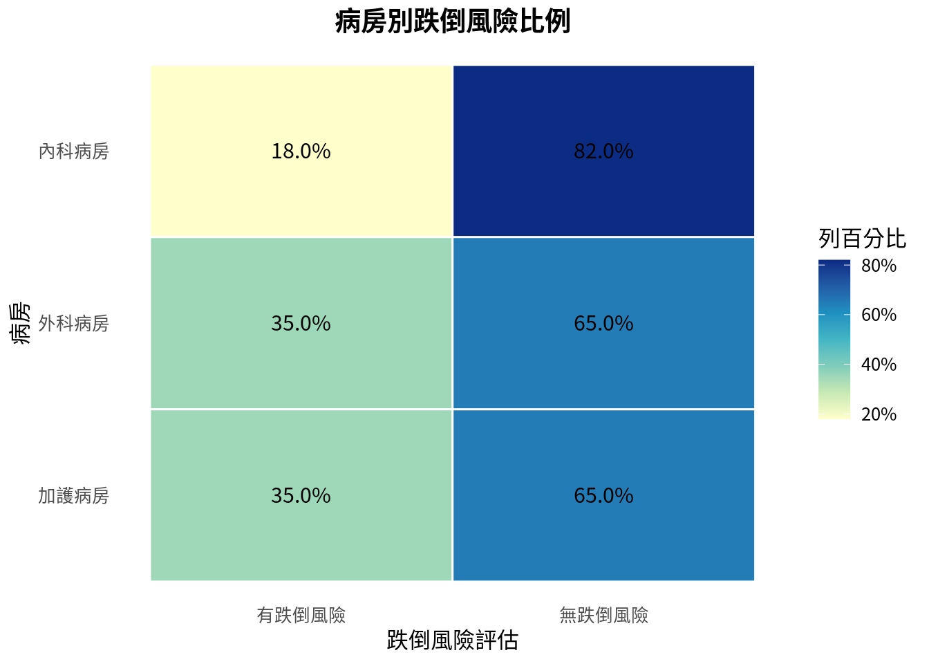
當兩個變項都是類別資料,可以放進列聯表 (contingency table)。例如「病房別」與「是否有跌倒風險」。
卡方獨立性檢定的虛無假設是兩個類別變項互相獨立。換句話說,跌倒風險比例不會因病房不同而不同。
範例 2:病房別跌倒風險是否不同?
ward_table <- data.frame(
  row.names = c("內科病房", "外科病房", "加護病房"),
  fall_risk = c(18, 35, 28),
  no_fall_risk = c(82, 65, 52),
  stringsAsFactors = FALSE
)
colnames(ward_table) <- c("有跌倒風險", "無跌倒風險")

ward_table
         有跌倒風險 無跌倒風險
內科病房         18         82
外科病房         35         65
加護病房         28         52
ward_percent <- ward_table / rowSums(ward_table)

ward_long <- ward_percent %>%
  rownames_to_column(var = "ward") %>%
  pivot_longer(cols = c("有跌倒風險", "無跌倒風險"), names_to = "fall_assessment", values_to = "percent")

ward_long$ward <- factor(ward_long$ward, levels = c("加護病房", "外科病房", "內科病房"))
ward_long$fall_assessment <- factor(ward_long$fall_assessment, levels = c("有跌倒風險", "無跌倒風險"))

p2 <- ggplot(ward_long, aes(x = fall_assessment, y = ward, fill = percent)) +
  geom_tile(color = "white", linewidth = 0.5) +
  geom_text(aes(label = sprintf("%.1f%%", percent * 100)), color = "black", size = 4) +
  scale_fill_distiller(palette = "YlGnBu", direction = 1, labels = scales::percent) +
  labs(
    title = "病房別跌倒風險比例",
    x = "跌倒風險評估",
    y = "病房",
    fill = "列百分比"
  ) +
  theme(panel.grid.major = element_blank(), panel.grid.minor = element_blank())

p2
chi2_result <- chisq.test(ward_table, correct = FALSE)

chi2_test_df <- data.frame(
  quantity = c("卡方統計量", "自由度", "p 值"),
  value = c(as.numeric(chi2_result$statistic), chi2_result$parameter, chi2_result$p.value),
  stringsAsFactors = FALSE
)
chi2_test_df$value <- round(chi2_test_df$value, 4)

chi2_test_df
    quantity  value
1 卡方統計量 9.0363
2     自由度 2.0000
3       p 值 0.0109
expected_df <- as.data.frame(chi2_result$expected)
rownames(expected_df) <- rownames(ward_table)
colnames(expected_df) <- colnames(ward_table)
round(expected_df, 2)
         有跌倒風險 無跌倒風險
內科病房      28.93      71.07
外科病房      28.93      71.07
加護病房      23.14      56.86
卡方檢定的一個重要檢查是期望次數 (expected count)。若期望次數太小,卡方近似可能不穩。常見經驗法則是大多數期望次數應至少 5;若 2x2 表中格子很小,Fisher exact test 通常更合適。
Fisher exact test:小樣本與稀有事件
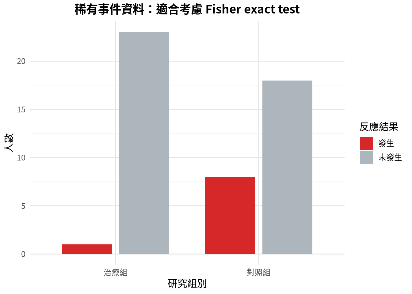
Fisher exact test 不依賴大樣本卡方近似,常用於 2x2 表,特別是事件很少的情境。它的計算較保守,但在小樣本時讓人睡得比較安穩。
範例 3:稀有嚴重不良事件
rare_table <- matrix(c(1, 8, 23, 18), nrow = 2, ncol = 2)
rownames(rare_table) <- c("治療組", "對照組")
colnames(rare_table) <- c("發生", "未發生")

rare_df <- data.frame(
  group = c("治療組", "治療組", "對照組", "對照組"),
  outcome = c("發生", "未發生", "發生", "未發生"),
  count = c(1, 23, 8, 18),
  stringsAsFactors = FALSE
)
rare_df$group <- factor(rare_df$group, levels = c("治療組", "對照組"))
rare_df$outcome <- factor(rare_df$outcome, levels = c("發生", "未發生"))

as.data.frame(rare_table)
p3 <- ggplot(rare_df, aes(x = group, y = count, fill = outcome)) +
  geom_col(position = position_dodge(width = 0.8), width = 0.7) +
  scale_fill_manual(values = c("發生" = "#d62828", "未發生" = "#adb5bd")) +
  labs(
    title = "稀有事件資料:適合考慮 Fisher exact test",
    x = "研究組別",
    y = "人數",
    fill = "反應結果"
  )

p3
fisher_result <- fisher.test(rare_table)
# 手算 sample odds ratio (ad/bc) 以與 SciPy 互通
odds_ratio_sample <- (rare_table[1,1] * rare_table[2,2]) / (rare_table[1,2] * rare_table[2,1])

fisher_test_df <- data.frame(
  quantity = c("勝算比", "雙尾 p 值"),
  value = c(odds_ratio_sample, fisher_result$p.value),
  stringsAsFactors = FALSE
)
fisher_test_df$value <- round(fisher_test_df$value, 4)

fisher_test_df
   quantity  value
1    勝算比 0.0978
2 雙尾 p 值 0.0244
Fisher exact test 在 R 的 fisher.test() 中會回傳勝算比估計與 p 值。若要正式報告,建議再加上勝算比信賴區間;本章先把重點放在檢定選擇與列聯表判讀。
McNemar test:配對二元資料
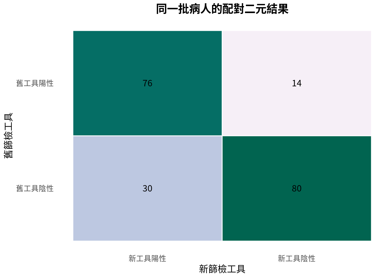
有些二元資料不是兩組獨立樣本,而是同一批人被測量兩次,或同一批檢體接受兩種檢測。例如同一批病人同時使用舊篩檢工具與新篩檢工具。這時不能用一般兩比例檢定,因為觀察值彼此配對。
McNemar test 的重點只看不一致的配對。若舊工具陽性新工具陰性的人數,和舊工具陰性新工具陽性的人數差很多,代表兩工具陽性率可能不同。
範例 4:新舊篩檢工具是否不同?
screen_table <- matrix(c(76, 30, 14, 80), nrow = 2, ncol = 2)
rownames(screen_table) <- c("舊工具陽性", "舊工具陰性")
colnames(screen_table) <- c("新工具陽性", "新工具陰性")

screen_df <- as.data.frame(screen_table)
screen_df
           新工具陽性 新工具陰性
舊工具陽性         76         14
舊工具陰性         30         80
screen_long <- screen_df %>%
  rownames_to_column(var = "old_tool") %>%
  pivot_longer(cols = c("新工具陽性", "新工具陰性"), names_to = "new_tool", values_to = "count")

screen_long$old_tool <- factor(screen_long$old_tool, levels = c("舊工具陰性", "舊工具陽性"))
screen_long$new_tool <- factor(screen_long$new_tool, levels = c("新工具陽性", "新工具陰性"))

p4 <- ggplot(screen_long, aes(x = new_tool, y = old_tool, fill = count)) +
  geom_tile(color = "white", linewidth = 0.5) +
  geom_text(aes(label = count), color = "black", size = 4) +
  scale_fill_distiller(palette = "PuBuGn", direction = 1) +
  labs(
    title = "同一批病人的配對二元結果",
    x = "新篩檢工具",
    y = "舊篩檢工具"
  ) +
  theme(
    legend.position = "none",
    panel.grid.major = element_blank(),
    panel.grid.minor = element_blank()
  )

p4
old_positive_new_negative <- screen_table[1, 2]
old_negative_new_positive <- screen_table[2, 1]
discordant_total <- old_positive_new_negative + old_negative_new_positive

mcnemar_p <- binom.test(
  min(old_positive_new_negative, old_negative_new_positive),
  discordant_total,
  p = 0.5
)$p.value

mcnemar_test_df <- data.frame(
  quantity = c("舊陽性新陰性", "舊陰性新陽性", "不一致配對總數", "exact McNemar p 值"),
  value = c(old_positive_new_negative, old_negative_new_positive, discordant_total, mcnemar_p),
  stringsAsFactors = FALSE
)
mcnemar_test_df$value <- round(mcnemar_test_df$value, 4)

mcnemar_test_df
            quantity   value
1       舊陽性新陰性 14.0000
2       舊陰性新陽性 30.0000
3     不一致配對總數 44.0000
4 exact McNemar p 值  0.0226
這裡用精確二項檢定實作 exact McNemar test。直覺是:在沒有差異的情況下,不一致配對應該差不多一半倒向舊工具、一半倒向新工具。
有序類別與趨勢檢定
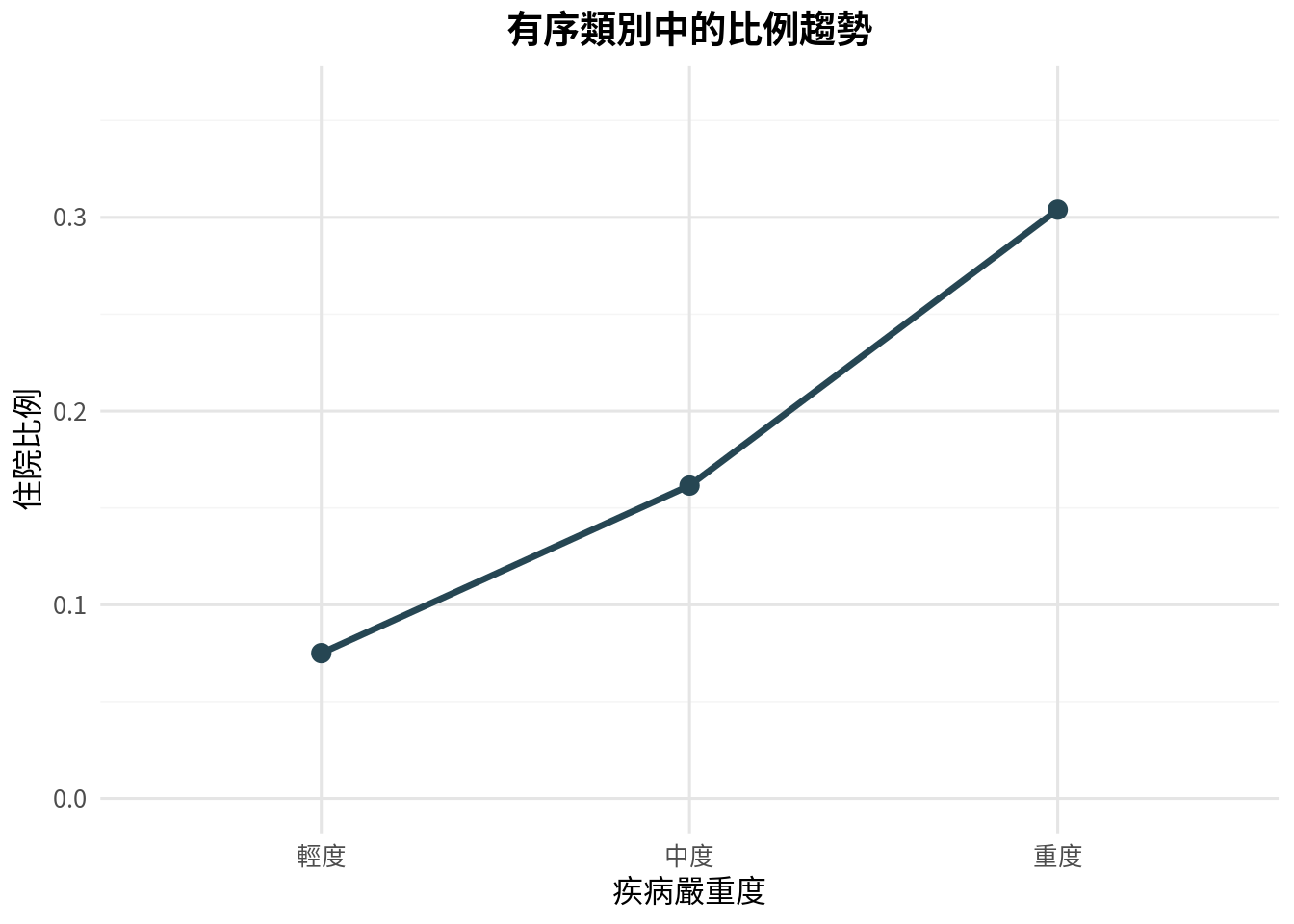
有些類別不是單純名目類別,而是有順序的,例如輕度、中度、重度。若結果是二元事件,可以問:事件比例是否隨類別順序增加或下降?
這類問題可使用 Cochran-Armitage trend test。在 R 語言中,可以安裝 coin 套件做類似處理。
範例 5:疾病嚴重度與住院比例
severity_df <- data.frame(
  severity = c("輕度", "中度", "重度"),
  score = c(1, 2, 3),
  events = c(9, 21, 38),
  total = c(120, 130, 125),
  stringsAsFactors = FALSE
)
severity_df$risk <- severity_df$events / severity_df$total

severity_df
  severity score events total      risk
1     輕度     1      9   120 0.0750000
2     中度     2     21   130 0.1615385
3     重度     3     38   125 0.3040000
severity_df$severity <- factor(severity_df$severity, levels = c("輕度", "中度", "重度"))

p5 <- ggplot(severity_df, aes(x = severity, y = risk, group = 1)) +
  geom_line(color = "#264653", linewidth = 1.2) +
  geom_point(color = "#264653", size = 3) +
  scale_y_continuous(limits = c(0, 0.36)) +
  labs(
    title = "有序類別中的比例趨勢",
    x = "疾病嚴重度",
    y = "住院比例"
  )

p5
cochran_armitage_trend <- function(successes, totals, scores) {
  successes <- as.numeric(successes)
  totals <- as.numeric(totals)
  scores <- as.numeric(scores)
  p_pool <- sum(successes) / sum(totals)
  score_bar <- sum(totals * scores) / sum(totals)
  numerator <- sum(scores * (successes - totals * p_pool))
  denominator <- sqrt(p_pool * (1 - p_pool) * sum(totals * (scores - score_bar)^2))
  z_stat <- numerator / denominator
  p_value <- 2 * (1 - pnorm(abs(z_stat)))
  return(list(z_stat = z_stat, p_value = p_value))
}

trend_res <- cochran_armitage_trend(
  severity_df$events,
  severity_df$total,
  severity_df$score
)

trend_test_df <- data.frame(
  quantity = c("趨勢 z 統計量", "雙尾 p 值"),
  value = c(trend_res$z_stat, trend_res$p_value),
  stringsAsFactors = FALSE
)
trend_test_df$value <- round(trend_test_df$value, 4)

trend_test_df
       quantity  value
1 趨勢 z 統計量 4.6589
2     雙尾 p 值 0.0000
趨勢檢定比一般卡方檢定更聚焦:它不是只問「三組是否有任何差異」,而是問「是否有隨順序上升或下降的線性趨勢」。當研究假設本來就有方向與順序時,這個問題更貼近臨床直覺。
常見錯誤
第一個錯誤是把配對資料當獨立資料。若同一位病人前後測、同一檢體做兩種檢測,就應考慮配對方法,例如 McNemar test。
第二個錯誤是只報告 p 值,不報告比例與效果大小。類別資料的效果大小可以是風險差、相對風險或勝算比。沒有這些數字,讀者很難知道差異是否有臨床意義。
第三個錯誤是小格子硬用卡方檢定。若事件很少,卡方近似可能不可靠。此時 Fisher exact test 或精確方法通常較合適。
第四個錯誤是忽略有序類別的順序。輕度、中度、重度不是三個任意標籤;若研究問題關心趨勢,應使用能保留順序資訊的方法。
本章重點整理
類別資料分析從計數開始。單一比例檢定處理一組比例與假設值的比較;兩比例 z 檢定處理兩個獨立比例的比較;卡方檢定處理兩個類別變項的關聯;Fisher exact test 適合小樣本 2x2 表;McNemar test 適合配對二元資料;趨勢檢定適合有序類別中的比例變化。
最好的報告方式不是「p = 0.03,所以有差」。比較成熟的寫法是:「疫苗組不良事件比例為 7.1%,對照組為 12.4%,風險差為 -5.3 個百分點,雙尾 p 值為 …」。數字一多,故事反而更清楚。
小練習
- 某篩檢計畫 300 人中有 42 人陽性。請檢定陽性率是否高於歷史值 10%。
- A 藥 180 人中有 24 人發生副作用,B 藥 175 人中有 39 人發生副作用。請計算兩組副作用比例、風險差與兩比例 z 檢定。
- 某研究有 3 個年齡層與是否接種疫苗的列聯表。你會用什麼檢定?若年齡層有明確順序,還能問什麼更聚焦的問題?
- 同一批 160 位病人使用兩種診斷工具,其中舊陽性新陰性為 18 人,舊陰性新陽性為 33 人。請用 exact McNemar test 判斷兩工具陽性率是否不同。
- 請解釋為什麼稀有事件資料不宜只依賴卡方近似。
# 練習 1
prac_events_1 <- 42
prac_total_1 <- 300
prac_p0_1 <- 0.10
res_1 <- binom.test(prac_events_1, prac_total_1, p = prac_p0_1, alternative = "greater")

# 練習 2
prac_a_events <- 24
prac_a_total <- 180
prac_b_events <- 39
prac_b_total <- 175
res_2 <- two_proportion_z_test(prac_a_events, prac_a_total, prac_b_events, prac_b_total)

# 練習 4
discordant_12 <- 18
discordant_21 <- 33
total_discordant <- discordant_12 + discordant_21
res_4_p <- binom.test(min(discordant_12, discordant_21), total_discordant, p = 0.5)$p.value

practice_results <- data.frame(
  問題 = c("篩檢陽性率單尾二項 p 值", "副作用風險差 (A-B)", "副作用檢定 z 統計量", "副作用檢定 p 值", "篩檢工具 exact McNemar p 值"),
  數值 = c(res_1$p.value, res_2$risk_diff, res_2$z_stat, res_2$p_value, res_4_p),
  stringsAsFactors = FALSE
)
practice_results$數值 <- round(practice_results$數值, 4)

practice_results
                         問題    數值
1     篩檢陽性率單尾二項 p 值  0.0166
2          副作用風險差 (A-B) -0.0895
3         副作用檢定 z 統計量 -2.2072
4             副作用檢定 p 值  0.0273
5 篩檢工具 exact McNemar p 值  0.0489
Glossary
| 類別資料 |
categorical data |
以類別而非連續數值表示的資料。 |
| 二元資料 |
binary data |
只有兩種結果的類別資料,例如是/否、陽性/陰性。 |
| 比例 |
proportion |
事件人數除以總人數。 |
| 風險 |
risk |
特定時間或情境下事件發生的機率或比例。 |
| 勝算 |
odds |
事件發生人數與未發生人數的比。 |
| 風險差 |
risk difference |
兩組風險相減。 |
| 相對風險 |
relative risk |
兩組風險相除。 |
| 勝算比 |
odds ratio |
兩組勝算相除。 |
| 列聯表 |
contingency table |
呈現兩個類別變項交叉計數的表格。 |
| 卡方獨立性檢定 |
chi-square test of independence |
檢定兩個類別變項是否獨立的方法。 |
| 期望次數 |
expected count |
虛無假設下,每個列聯表格子預期的計數。 |
| Fisher 精確檢定 |
Fisher exact test |
用於 2x2 表的小樣本精確檢定。 |
| McNemar 檢定 |
McNemar test |
用於配對二元資料的檢定。 |
| 趨勢檢定 |
trend test |
檢定有序類別中事件比例是否呈現上升或下降趨勢的方法。 |