本章學習目標
前面的章節多半從「已經有一張資料表」開始,然後討論如何估計、檢定與建模。流行病學研究多了一個很重要的問題:這張資料表是怎麼來的?研究設計 (study design) 會決定可以估計什麼效果量、容易受到哪些偏差影響,以及結果能不能合理解讀為因果線索。
本章介紹常見流行病學研究設計與分析技巧,包括 cohort study、case-control study、cross-sectional study、風險比、勝算比、混雜、分層與標準化。這些概念是公共衛生與臨床研究的地基。地基歪了,後面模型蓋得再漂亮也會讓人心裡很緊。
讀完本章後,你應該能夠:
區分 cohort、case-control 與 cross-sectional study。
解釋 incidence、prevalence、risk、rate 的差異。
計算並解讀 risk ratio、odds ratio 與 risk difference。
說明 case-control study 為什麼通常估計 odds ratio。
使用分層分析檢查混雜與效果修飾。
理解 Mantel-Haenszel adjustment 的基本直覺。
說明直接標準化 (direct standardization) 的目的。
辨認 selection bias、information bias 與 confounding。
三種常見研究設計
Cohort study 從暴露狀態出發,追蹤未來是否發生結果。例如先分成吸菸與未吸菸,再追蹤心血管事件。它可以直接估計發生風險與 incidence rate,時間順序也比較清楚。
Case-control study 從疾病狀態出發,回頭比較過去暴露。例如先找肺癌病例與非肺癌對照,再比較過去吸菸比例。它適合罕見疾病或潛伏期很長的疾病,但通常不能直接估計風險,只能估計 odds ratio。
Cross-sectional study 在同一時間點測量暴露與結果。例如同一天調查是否久坐與是否有高血壓。它適合估計盛行率 (prevalence),但時間順序較不清楚。
簡單整理如下:
Cohort study
暴露狀態
Risk ratio, rate ratio
可看時間順序,可估 incidence
費時,罕見疾病效率低
Case-control study
疾病狀態
Odds ratio
適合罕見疾病,效率高
選擇對照與回憶偏差很關鍵
Cross-sectional study
同一時間點
Prevalence ratio, odds ratio
快速估盛行率
時間順序不明
Incidence 與 prevalence
Incidence 描述新發生事件。若 1,000 位原本沒有疾病的人追蹤一年後有 50 位發病,累積發生風險是 5%。如果每個人的追蹤時間不同,就常用 incidence rate,也就是事件數除以人時 (person-time)。
Prevalence 描述某一時間點或期間「已經有疾病」的比例。例如某社區今天有 8% 成人有糖尿病,這是盛行率。Prevalence 受 incidence 與疾病持續時間影響;慢性病即使 incidence 不高,也可能有高 prevalence。
不要把 incidence 與 prevalence 混在一起。Incidence 比較像「新病人進來的速度」,prevalence 比較像「病房現在住了多少人」。兩者都重要,但回答的問題不同。
Cohort study:從暴露追蹤結果
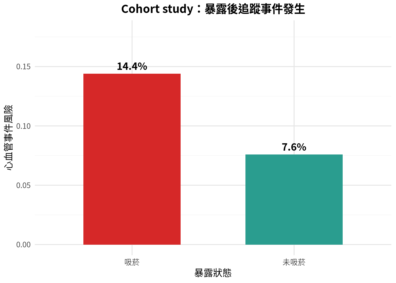
假設我們追蹤 1,000 位成人,依基線吸菸狀態分成吸菸與未吸菸各 500 人,觀察 5 年內是否發生心血管事件。
<- data.frame (exposure = c ("吸菸" , "吸菸" , "未吸菸" , "未吸菸" ),outcome = c ("發生心血管事件" , "未發生" , "發生心血管事件" , "未發生" ),count = c (72 , 428 , 38 , 462 ),stringsAsFactors = FALSE
  exposure        outcome count
1     吸菸 發生心血管事件    72
2     吸菸         未發生   428
3   未吸菸 發生心血管事件    38
4   未吸菸         未發生   462
<- data.frame (exposure = factor (c ("吸菸" , "未吸菸" ), levels = c ("吸菸" , "未吸菸" )),events = c (72 , 38 ),total = c (500 , 500 ),stringsAsFactors = FALSE $ risk <- cohort_risk$ events / cohort_risk$ total<- ggplot (cohort_risk, aes (x = exposure, y = risk, fill = exposure)) + geom_col (show.legend = FALSE , width = 0.6 ) + geom_text (aes (label = sprintf ("%.1f%%" , risk * 100 )), vjust = - 0.5 , size = 4.5 , fontface = "bold" ) + scale_fill_manual (values = c ("吸菸" = "#d62828" , "未吸菸" = "#2a9d8f" )) + scale_y_continuous (limits = c (0 , 0.18 )) + labs (title = "Cohort study:暴露後追蹤事件發生" ,x = "暴露狀態" ,y = "心血管事件風險"
<- function (a, b, c, d) {<- a / (a + b)<- c / (c + d)<- risk_exposed / risk_unexposed<- sqrt (1 / a - 1 / (a + b) + 1 / c - 1 / (c + d))<- exp (log (rr) + c (- 1.96 , 1.96 ) * se_log)return (list (rr = rr, ci = ci, risk_exposed = risk_exposed, risk_unexposed = risk_unexposed))
<- risk_ratio_ci (72 , 428 , 38 , 462 )<- res_rr$ risk_exposed - res_rr$ risk_unexposed<- data.frame (quantity = c ("吸菸組風險" , "未吸菸組風險" , "風險差" , "風險比" , "風險比 95% CI 下限" , "風險比 95% CI 上限" ),value = c (res_rr$ risk_exposed, res_rr$ risk_unexposed, risk_difference, res_rr$ rr, res_rr$ ci[1 ], res_rr$ ci[2 ]),stringsAsFactors = FALSE $ value <- round (rr_output_df$ value, 4 )
            quantity  value
1         吸菸組風險 0.1440
2       未吸菸組風險 0.0760
3             風險差 0.0680
4             風險比 1.8947
5 風險比 95% CI 下限 1.3049
6 風險比 95% CI 上限 2.7512
風險比 (risk ratio, RR) 約為 1.89,表示吸菸組 5 年心血管事件風險約為未吸菸組的 1.89 倍。風險差則約為 6.8 個百分點,回答的是絕對差異。臨床與公共衛生決策常常需要兩者一起看:相對效果很醒目,絕對效果才更接近資源配置。
Case-control study:從疾病回看暴露
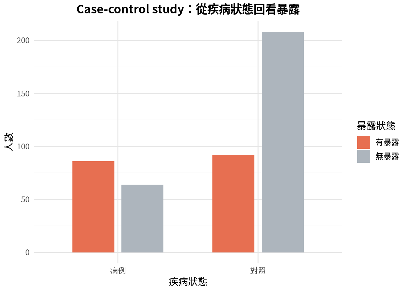
Case-control study 先選病例與對照,再回頭比較暴露比例。因為病例與對照人數通常是研究者抽樣決定的,所以不能直接用病例比例估計疾病風險。此時常用勝算比 (odds ratio, OR)。
<- data.frame (disease = c ("病例" , "病例" , "對照" , "對照" ),exposure = c ("有暴露" , "無暴露" , "有暴露" , "無暴露" ),count = c (86 , 64 , 92 , 208 ),stringsAsFactors = FALSE $ disease <- factor (case_control_table$ disease, levels = c ("病例" , "對照" ))$ exposure <- factor (case_control_table$ exposure, levels = c ("有暴露" , "無暴露" ))
  disease exposure count
1    病例   有暴露    86
2    病例   無暴露    64
3    對照   有暴露    92
4    對照   無暴露   208
<- ggplot (case_control_table, aes (x = disease, y = count, fill = exposure)) + geom_col (position = position_dodge (width = 0.7 ), width = 0.6 ) + scale_fill_manual (values = c ("有暴露" = "#e76f51" , "無暴露" = "#adb5bd" )) + labs (title = "Case-control study:從疾病狀態回看暴露" ,x = "疾病狀態" ,y = "人數" ,fill = "暴露狀態"
<- function (a, b, c, d) {<- (a * d) / (b * c)<- sqrt (1 / a + 1 / b + 1 / c + 1 / d)<- exp (log (or_value) + c (- 1.96 , 1.96 ) * se_log)return (list (or_value = or_value, ci = ci))
<- odds_ratio_ci (86 , 64 , 92 , 208 )<- data.frame (quantity = c ("勝算比" , "95% CI 下限" , "95% CI 上限" ),value = c (res_or$ or_value, res_or$ ci[1 ], res_or$ ci[2 ]),stringsAsFactors = FALSE $ value <- round (or_output_df$ value, 4 )
     quantity  value
1      勝算比 3.0380
2 95% CI 下限 2.0241
3 95% CI 上限 4.5600
若疾病罕見,OR 會接近 RR。若疾病常見,OR 可能明顯高估 RR 的大小。報告時應清楚說是 odds ratio,不要自動說成「風險增加幾倍」。
效果量圖:RR 與 OR
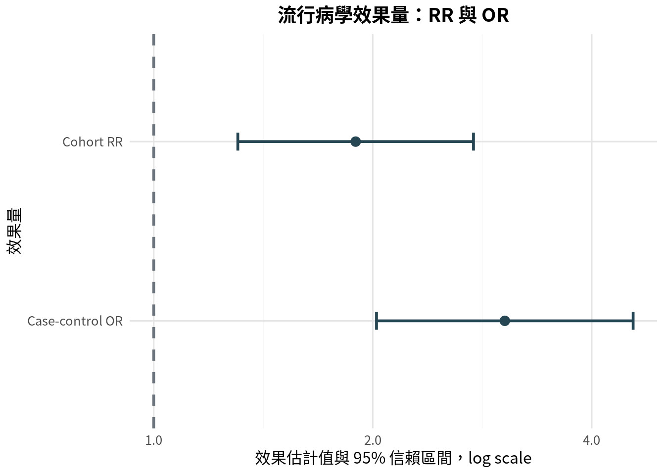
森林圖 (forest plot) 常用來呈現效果量與信賴區間。RR 與 OR 的虛無值都是 1,因此圖上常畫一條垂直線在 1。
<- data.frame (measure = factor (c ("Cohort RR" , "Case-control OR" ), levels = c ("Case-control OR" , "Cohort RR" )),estimate = c (res_rr$ rr, res_or$ or_value),lower = c (res_rr$ ci[1 ], res_or$ ci[1 ]),upper = c (res_rr$ ci[2 ], res_or$ ci[2 ]),stringsAsFactors = FALSE <- ggplot (effect_df, aes (x = estimate, y = measure)) + geom_errorbar (aes (xmin = lower, xmax = upper), width = 0.1 , color = "#264653" , linewidth = 1 ) + geom_point (color = "#264653" , size = 3 ) + geom_vline (xintercept = 1 , color = "#6c757d" , linetype = "dashed" , linewidth = 1 ) + scale_x_log10 (breaks = c (0.5 , 1 , 2 , 4 ), labels = c ("0.5" , "1.0" , "2.0" , "4.0" )) + labs (title = "流行病學效果量:RR 與 OR" ,x = "效果估計值與 95% 信賴區間,log scale" ,y = "效果量"
使用 log scale 是因為 RR 與 OR 的信賴區間在乘法尺度上比較自然,也能讓小於 1 與大於 1 的效果呈現較對稱。
混雜與分層分析
混雜因子 (confounder) 是同時與暴露及結果相關、且不在暴露到結果因果路徑上的變項。年齡是醫學研究中最常見的混雜因子之一。若用藥組病人較年長,而年齡本身也增加事件風險,未調整的用藥效果可能被年齡混雜。
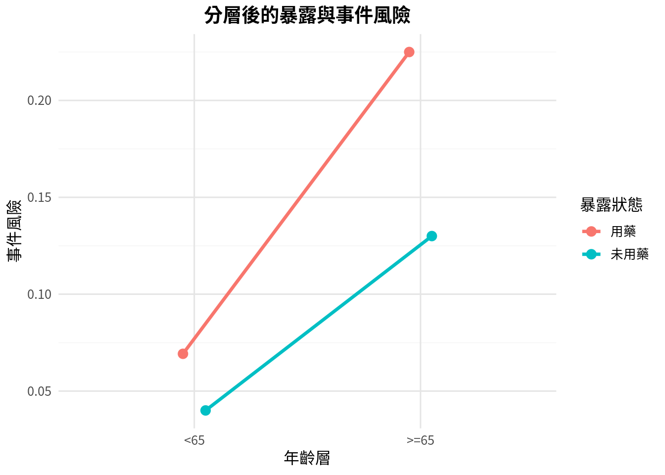
分層分析 (stratified analysis) 是處理混雜的基本方法:先在每個年齡層內比較暴露與結果,再看各層效果是否一致。
<- data.frame (age_group = c ("<65" , "<65" , ">=65" , ">=65" ),exposure = c ("用藥" , "未用藥" , "用藥" , "未用藥" ),events = c (18 , 12 , 54 , 26 ),total = c (260 , 300 , 240 , 200 ),stringsAsFactors = FALSE $ risk <- strata_df$ events / strata_df$ total$ age_group <- factor (strata_df$ age_group, levels = c ("<65" , ">=65" ))$ exposure <- factor (strata_df$ exposure, levels = c ("用藥" , "未用藥" ))
  age_group exposure events total       risk
1       <65     用藥     18   260 0.06923077
2       <65   未用藥     12   300 0.04000000
3      >=65     用藥     54   240 0.22500000
4      >=65   未用藥     26   200 0.13000000
<- ggplot (strata_df, aes (x = age_group, y = risk, color = exposure, group = exposure)) + geom_line (position = position_dodge (width = 0.2 ), linewidth = 1.2 ) + geom_point (position = position_dodge (width = 0.2 ), size = 3 ) + labs (title = "分層後的暴露與事件風險" ,x = "年齡層" ,y = "事件風險" ,color = "暴露狀態"
<- list ()<- 1 for (age_grp in levels (strata_df$ age_group)) {<- strata_df %>% filter (age_group == age_grp & exposure == "用藥" )<- strata_df %>% filter (age_group == age_grp & exposure == "未用藥" )<- risk_ratio_ci ($ events,$ total - exposed$ events,$ events,$ total - unexposed$ events<- data.frame (age_group = age_grp,risk_exposed = res_layer$ risk_exposed,risk_unexposed = res_layer$ risk_unexposed,risk_ratio = res_layer$ rr,lower = res_layer$ ci[1 ],upper = res_layer$ ci[2 ],stringsAsFactors = FALSE <- idx + 1 <- do.call (rbind, stratum_results)%>% mutate (across (c (risk_exposed, risk_unexposed, risk_ratio, lower, upper), ~ round (., 4 )))
  age_group risk_exposed risk_unexposed risk_ratio  lower  upper
1       <65       0.0692           0.04     1.7308 0.8498 3.5250
2      >=65       0.2250           0.13     1.7308 1.1275 2.6569
若各層風險比相近,但與粗略風險比不同,代表可能有混雜。若各層風險比差很多,可能存在效果修飾 (effect modification),也就是暴露效果在不同年齡層真的不一樣。混雜通常想調整;效果修飾通常想報告。
Mantel-Haenszel adjustment 的直覺
Mantel-Haenszel 方法可把各層資訊加權合併,得到調整後效果估計。它不是魔法,只是讓每一層在自己的比較中貢獻資訊,避免年齡分布不同直接扭曲暴露效果。
<- function (strata) {<- 0.0 <- 0.0 for (i in seq_along (strata)) {<- strata[[i]]<- row$ a<- row$ b<- row$ c<- row$ d<- a + b + c + d<- numerator + a * (c + d) / n<- denominator + c * (a + b) / nreturn (numerator / denominator)<- list (list (a = 18 , b = 242 , c = 12 , d = 288 ),list (a = 54 , b = 186 , c = 26 , d = 174 )<- mantel_haenszel_rr (strata_list)<- data.frame (quantity = c ("Mantel-Haenszel adjusted RR" ),value = c (mh_rr),stringsAsFactors = FALSE $ value <- round (mh_df$ value, 4 )
                     quantity  value
1 Mantel-Haenszel adjusted RR 1.7308
在更複雜的研究中,我們常用 regression model 進行調整,例如 logistic regression、Poisson regression 或 Cox regression。但分層分析仍是非常重要的第一步,因為它讓資料結構被看見,而不是全部塞進模型後就假裝世界很單純。
標準化:讓族群結構可比較
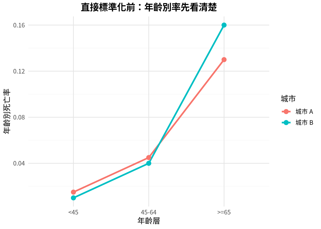
比較兩個城市死亡率時,如果城市 A 較年輕、城市 B 較老,粗死亡率可能主要反映年齡結構,而不是醫療品質或疾病風險差異。直接標準化 (direct standardization) 使用同一個標準人口年齡分布,計算若兩城市有相同年齡結構時的預期率。
<- data.frame (age_group = c ("<45" , "45-64" , ">=65" ),standard_n = c (5000 , 3000 , 2000 ),city_a_rate = c (0.015 , 0.045 , 0.13 ),city_b_rate = c (0.010 , 0.040 , 0.16 ),stringsAsFactors = FALSE $ city_a_expected <- standard_population$ standard_n * standard_population$ city_a_rate$ city_b_expected <- standard_population$ standard_n * standard_population$ city_b_rate
  age_group standard_n city_a_rate city_b_rate city_a_expected city_b_expected
1       <45       5000       0.015        0.01              75              50
2     45-64       3000       0.045        0.04             135             120
3      >=65       2000       0.130        0.16             260             320
<- standard_population %>% pivot_longer (cols = c (city_a_rate, city_b_rate), names_to = "city" , values_to = "rate" ) %>% mutate (city = recode (city, "city_a_rate" = "城市 A" , "city_b_rate" = "城市 B" ))$ age_group <- factor (std_plot$ age_group, levels = c ("<45" , "45-64" , ">=65" ))<- ggplot (std_plot, aes (x = age_group, y = rate, color = city, group = city)) + geom_line (linewidth = 1.2 ) + geom_point (size = 3 ) + labs (title = "直接標準化前:年齡別率先看清楚" ,x = "年齡層" ,y = "年齡別死亡率" ,color = "城市"
<- sum (standard_population$ city_a_expected) / sum (standard_population$ standard_n)<- sum (standard_population$ city_b_expected) / sum (standard_population$ standard_n)<- data.frame (city = c ("城市 A" , "城市 B" ),direct_standardized_rate = c (direct_a, direct_b),stringsAsFactors = FALSE $ direct_standardized_rate <- round (std_rates_df$ direct_standardized_rate, 4 )
    city direct_standardized_rate
1 城市 A                    0.047
2 城市 B                    0.049
標準化不是讓城市變公平,而是讓比較更公平。它控制的是已知且可分層的族群結構,例如年齡、性別。若有未測量混雜,標準化仍無法解決。
偏差:不是 p 值可以修好的問題
Selection bias 發生在研究對象進入研究的方式與暴露或結果有關。例如病例對照研究中,對照組若不是來自能產生病例的同一來源族群,OR 可能偏掉。
Information bias 來自測量錯誤或分類錯誤。例如病例比對照更努力回想過去暴露,可能造成 recall bias。若暴露或結果測量不準確,再精細的模型也只是精準地分析一張有問題的表。
Confounding 則是第三變項造成暴露與結果關係混淆。它可以透過設計處理,例如 randomization、restriction、matching,也可以透過分析處理,例如 stratification、standardization、regression adjustment。
研究設計階段能避免的偏差,不要留到分析階段才祈禱。統計方法很能幹,但不是時光機。
常見錯誤
第一個錯誤是把 case-control study 的 OR 解讀成風險比。病例與對照人數通常由研究設計決定,不能直接估計疾病風險。
第二個錯誤是只報相對效果,不報絕對風險。RR = 2 可以很驚人,但若基準風險從 0.1% 到 0.2%,公共衛生意義與從 10% 到 20% 不一樣。
第三個錯誤是看到調整後模型就放心。調整只能處理有測量且放入模型的混雜因子,也依賴模型形式合理。
第四個錯誤是把效果修飾當成麻煩。其實效果修飾常常是臨床上最有意思的發現:同一介入可能對不同族群效果不同。
第五個錯誤是忽略研究對象來源。外部效度與選擇偏差都和「誰被納入研究」密切相關。
本章重點整理
流行病學分析必須先理解研究設計。Cohort study 從暴露追蹤結果,適合估計風險與風險比;case-control study 從疾病狀態回看暴露,常估計勝算比;cross-sectional study 同時測量暴露與結果,適合估計盛行率。
效果量比 p 值更接近研究問題。RR、OR、risk difference、prevalence ratio 都有自己的適用情境。混雜、偏差與效果修飾則提醒我們:資料不是從天上掉下來的,它有來源、有路徑,也有脾氣。
小練習
某研究從 2,000 位無疾病成人開始追蹤 10 年,依是否暴露於空氣污染分組。這是什麼研究設計?可估計哪些效果量?
某研究選 300 位罕見癌症病例與 600 位對照,回顧過去職業暴露。為什麼此研究通常報告 OR 而不是 RR?
請用自己的話解釋 incidence 與 prevalence 的差異。
若粗 RR 為 2.0,但年齡分層後每一層 RR 都約為 1.2,你會懷疑什麼?
若年輕層 RR 為 1.0,老年層 RR 為 2.5,這比較像混雜還是效果修飾?為什麼?
請舉一個 selection bias 與一個 information bias 的醫學研究例子。
Glossary
研究設計
study design
研究對象、暴露、結果與時間順序的安排方式。
世代研究
cohort study
從暴露狀態出發,追蹤結果發生的研究設計。
病例對照研究
case-control study
從疾病狀態出發,回顧暴露狀態的研究設計。
橫斷面研究
cross-sectional study
在同一時間點測量暴露與結果的研究設計。
發生率
incidence
新發生事件的頻率。
盛行率
prevalence
某時間點或期間已有疾病的比例。
風險
risk
一定期間內事件發生的機率或比例。
率
rate
事件數除以人時的發生率。
風險比
risk ratio
兩組風險的比值。
風險差
risk difference
兩組風險的差值。
勝算比
odds ratio
兩組勝算的比值。
混雜因子
confounder
同時與暴露及結果相關、可能扭曲關係估計的變項。
分層分析
stratified analysis
依第三變項分層後進行分析的方法。
效果修飾
effect modification
暴露效果因另一變項水準不同而改變的現象。
Mantel-Haenszel 調整
Mantel-Haenszel adjustment
將分層效果量加權合併的調整方法。
直接標準化
direct standardization
使用標準人口結構計算可比較率的方法。
選擇偏差
selection bias
研究對象選入方式造成的偏差。
資訊偏差
information bias
測量或分類錯誤造成的偏差。